Optimizing HPLC/UHPLC Systems
Just for Fun – Explain the Difference
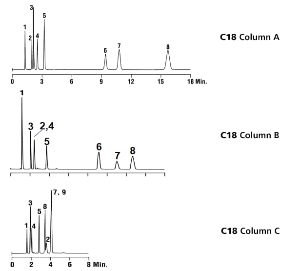
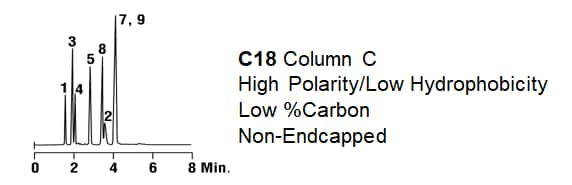
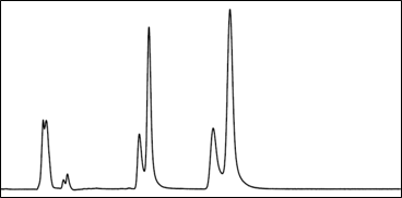
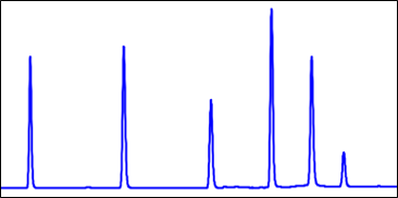
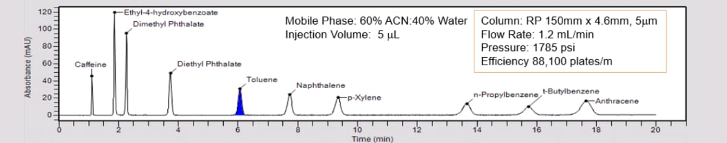
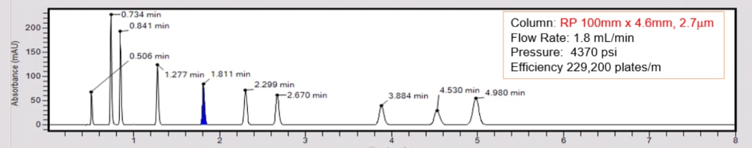
Look at the three chromatograms below.
- They are all performed with “C18” column chemistries.
- The same 8 component test mix was injected on each column.
- All 3 separations are performed using the same mobile phase.
- All 3 columns have the same hardware format (length, width).
- All 3 columns are packed with the same particle size stationary phase.
How can it be? How can the results be so different?
|
1. Uracil 2. 3-butylpyridine 3. Phenol 4. 4-phenylbutyric acid 5. N,N-diethyl-meta-toluamide (DEET) 6. Quinizarin |
7. Propylbenzene 8. Butylbenzene |
|
Mobile Phase: 25mM KH2PO4 pH 2.5:ACN (35:65) Flow Rate: 1.0mL/min Detector: UV at 254nm |
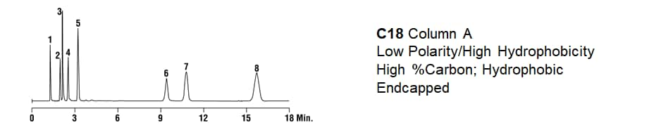
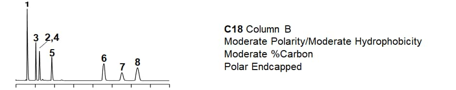
The answer lies in the bonded phase chemistry of the packed bed. The columns each have a different % carbon loading (bonded phase coverage on the silica) and a different kind of end-capping. Vastly different results. Proof that a C18 is not a C18 is not a C18.
General Recommendations
- Plumb systems with 0.005” tubing or smaller ID
- Keep injected volumes between 1 and 5µL (~1% of void volume)
- Always use high quality HPLC-grade or UHPLC-grade mobile phase solvents.
- Consider pre-filtering mobile phase solvents through 0.45µm filters, especially after modification with a buffer
- Always pre-filter samples through 0.45µm or 0.2µm syringe filters or use filter vials that provide the same function.
- Consider a 100 x 3mm pack with 2.7 μm SPP particles for quality HPLC
- higher efficiency than standard HPLC
- lower back pressure than 3 μm traditional particles
- more resistant to clogging than traditional particles
- Consider a 50 x 2.1mm packed with sub-2µm particles optimal for UHPLC
- comparable theoretical plates, N, to a 150 x 4.6mm, 5µm
- optimal flows in the range 300 – 600µL/min
- run times from 3 – 5min. (100 x 2.1mm, 7 – 10min.)
- back pressure will be higher
Contributions to band broadening
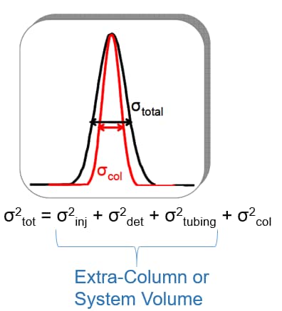
- Injector mechanism
- Detector flow cell
- Connection tubing between injector and column
- Connection tubing between column and detector flow cell
The smaller the intra-column volume, the higher the contribution from extra-column volume
Good UHPLC performance demands that we minimize the system volume by using minimum tubing IDs and the shortest lengths.
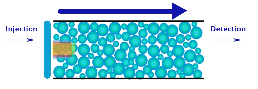
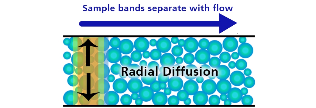
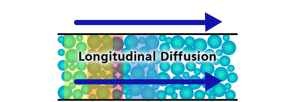
Animation Explanation
Too much extra-column volume will result in peak broadening. This is called dispersion. Perceived chromatographic resolution will be lower and detector sensitivity will be lower because of reduced peak height.
Optimizing for Delay Volume
Vd = Vmixer + Vinj + Vtubing
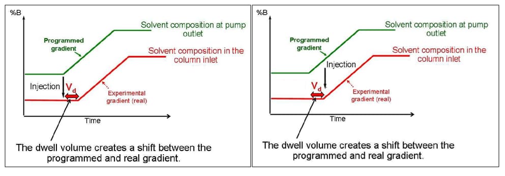
Gradient Delay volume is the total amount of volume from the point of mixing to the head of the column.
- No affect on isocratic separations
- Significant affect on gradient separations when the column volume is small. Gradient delay is how long it takes a gradient to hit the head of the column.
- A gradient delay volume of 200uL on a system flowing at 200uL/min. will produce a gradient delay of 1min. That’s 1 minute of chromatography with no gradient on the column.
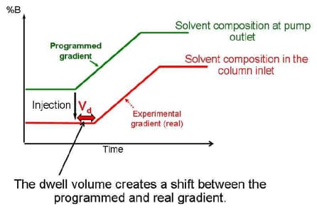
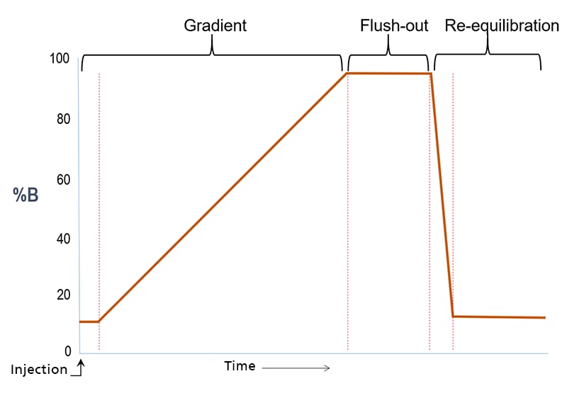
Gradient Delay or “Dwell” Volume
-
-
Gradient Delay Volume (Vd) in RED
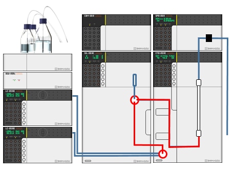
Gradient delay is most noticeable with small-volume LC columns. As a practical example consider a 100 x 2.1mm column operating at a flow rate of 200 μL/min on a system with 200 μL of delay volume. It would take 1 minute for the column to “see” the gradient –the first minute would be initial isocratic condition. That “1 minute” may be 20% or more of the run time.
Compensating for Gradient Delay
- Consider using an injection delay so that the injection is performed at the same instant as the gradient hitting the column.
- The pump program will start before the injection is performed.
- This can be used to compensate for “dwell volume” differences between different HPLC systems.
Practical Method Considerations
- Proper column flush and equilibration are key to reproducibility.
- “By the book”, 10 column volumes of flow are necessary for complete packed-bed equilibration.
| Title | Void Volume | Eq. Time @400µL/min. |
|---|---|---|
| 50 x 2.1mm, 1.9µm | 0.1mL | 0.25min |
| 100 x 2.1mm, 1.9µm | 0.2mL | 0.5min |
Sample Matrix Strength
- Be conscious of the elution strength of the sample’s solvent matrix. In general, make sure the sample matrix is no “stronger” than the chromatography mobile phase condition at the time of injection.
- A sample matrix that is too “strong” relative to the mobile phase at time of injection can hinder the separation of sample constituents through a pre-elution effect. Sample partitioning into the stationary phase bed is hindered if the injection solvent is too strong relative to the mobile phase.
|
MP A: Water MP B: Acetonitrile Gradient: 10 – 100% B over 5 minutes Sample Matrix: 100% Acetonitrile |
MP A: Water MP B: Acetonitrile Gradient: 5 – 100% B over 5 minutes Sample Matrix: 10% Acetonitrile in Water |
|---|---|
 |
 |
Some Basic HPLC Flow Principles
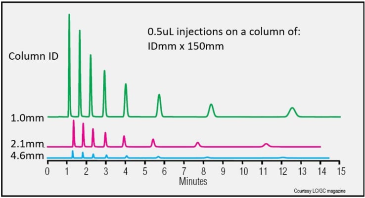
Detector Response and Column ID
Reducing the column ID ( ↓ radial diffusion ) increases the peak height/sensitivity:
- Sensitivity increases as (Δ ID)2
- 4.6mm - > 2.1mm results in ~ 5-fold sensitivity increase
- 4.6mm - > 1.0mm results in ~ 21-fold sensitivity increase
Solvent Consumption and Column ID
| Column format | Solvent Consumed in five 20min. Runs* | Reduction in solvent used |
|---|---|---|
| 4.6 x 150mm | 100mL | 0 |
| 3.0 x 150mm | 42mL | 58% |
| 2.1 x 150mm | 13mL | 87% |
* Flow rate = 1mL/min.
Choosing HPLC/UHPLC Columns
Choose columns according to analysis goals (sample throughput, resolution, target chemistries)
- Particle mechanics – particle size, fully- or superficially porous
- Column format – length and ID
- Chemistry – According to the chemistry of the sample constituents
SPP – Superficially Porous Particles
- Better uniformity of particle size results in reduced pressure drop for the same flow rate
- Comparable or better resolving power to non-SPP with same particle size
- Robust and forgiving (does not clog as easily as columns packed with sub-2µm materials
- Available in 2.7µm particles
- Good way to get better chromatographic efficiency out of a standard HPLC system
2.7µm Superficially Porous Particles offer high resolution and fast separations approaching that of UHPLC but without the higher backpressures.
Isocratic vs. Gradient Elution Modes
Isocratic Elution
- A single composition of solvents is used for the duration of the separation
- Later eluting peaks are broader than earlier eluting peaks because of dispersion effects on the column at a constant flow rate
- Steps must be taken to periodically flush the column at higher solvent strength to clean it of intractable materials that build up from sample injections
Gradient Elution
- The composition of solvents is changed either continuously or stepwise
- In general, peaks are sharper throughout the chromatogram when compared to isocratic elution
- Some separations may be achieved which are not possible using isocratic elution
- Chromatogram run times may be shorter when compared to isocratic elution
Method Development – Suggested Screening Gradient
Recommended LC Column:
- Column Chemistry: e.g. C18, C8, C4, Phenyl-Hexyl, Biphenyl
- Column Format: 100 x 3 mm, 2.7 to 5 µm particles
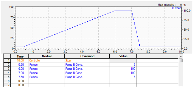
Shimadzu LabSolutions Pump Program – Screening Gradient
Screening Gradient
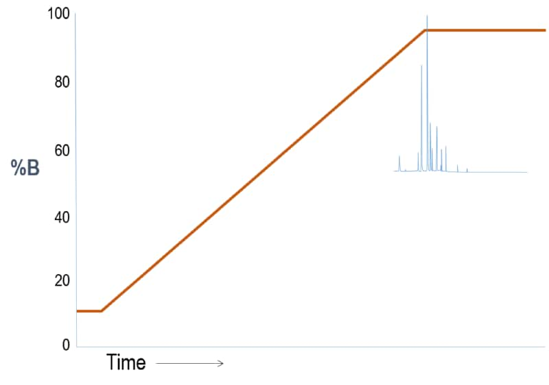
Outcome Scenario #1: Gradient Elution (Weak “A” – Strong “B” solvent system)
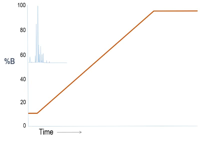
Interpretation
For a reversed phase LC column where A is water and B is organic, this first run shows sample constituents that are all polar. So, the separation is poor because the substances experience little partitioning on the stationary phase. In other words, the weak, starting solvent condition brings the sample constituents off too early.
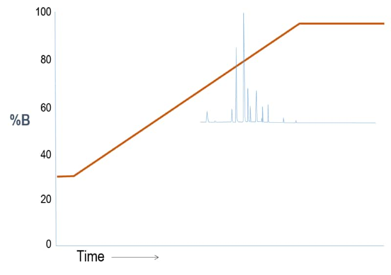
Outcome Scenario #1: Gradient Elution (Weak “A” – Strong “B” solvent system)
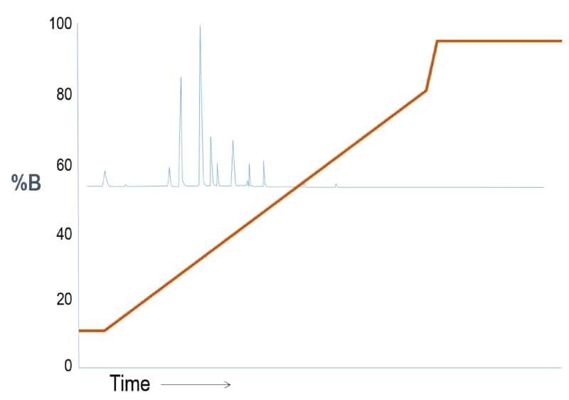
Interpretation
To cause the substances to partition more into the stationary phase, we reduce the slope of the gradient so that the mobile phase strength does not increase as quickly. The substances retain longer and begin to separate from one another. Notice that we still “flush” the column with strong solvent at the end of the run to effectively clean the column.
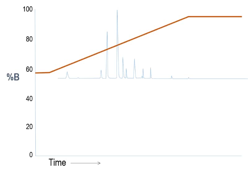
Outcome Scenario #1: Gradient Elution (Weak “A” – Strong “B” solvent system)
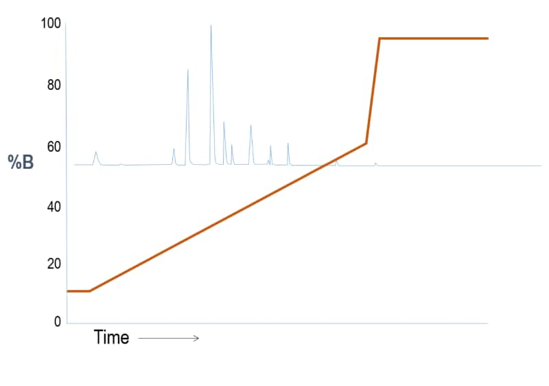
Interpretation
We reduce the gradient slope again until we begin seeing a good separation within the time frame.
Outcome Scenario #2: Gradient Elution (Weak “A” – Strong “B” solvent system)
Interpretation
For a reversed phase LC column where A is water and B is organic, this first run shows sample constituents that are all very non-polar. So, the separation is poor because the substances come off late –only when the solvent strength is high.
Outcome Scenario #2: Gradient Elution (Weak “A” – Strong “B” solvent system)
Interpretation
Here, we start the gradient run at a higher solvent strength so the sample constituents begin partitioning into the stationary phase earlier.
Outcome Scenario #2: Gradient Elution (Weak “A” – Strong “B” solvent system)
Interpretation
Again, the gradient is adjusted to start at a higher solvent strength so the sample constituents begin partitioning into the stationary phase earlier.
